SDR Classifier
I was recently involved in the porting of NuPIC’s SDR Classifier to Java, for the HTM.Java project. When I began the process, I knew pretty much nothing about the SDR Classifier or neural networks. So, I took extensive notes while I learned about them. I’ve decided to curate my notes and present them in this blog post, in the hope that they will prove useful. So, without further ado:
What Is It?
The purpose of the SDR Classifier is identical to that of the CLA Classifier: learn associations between a given state of the Temporal Memory at time \(t\), and the value that is to be fed into the Encoder at time \(t + n\) (where \(n\) is the number of steps into the future you want to predict. \(t + 1\), \(t + 5\), \(t + 2\) - or all three!). You can also think of it as mapping activation patterns (vector of Temporal Memory’s active cells) to probability distributions (for the possible encoder buckets).
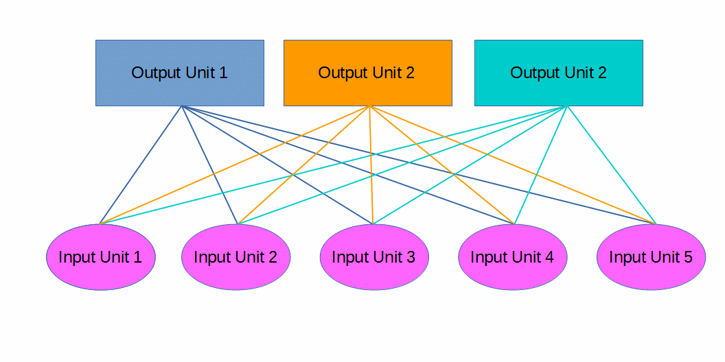
The SDR Classifier accomplishes this by implementing a single layer, feed forward, neural network. The network has “output units” (neurons in the network) and “input units” (bits in the activation pattern - the vector of Temporal Memory’s active cells). The number of output units is equal to the number of buckets the encoder uses. The number of input units is simply the number of bits in the activation pattern.
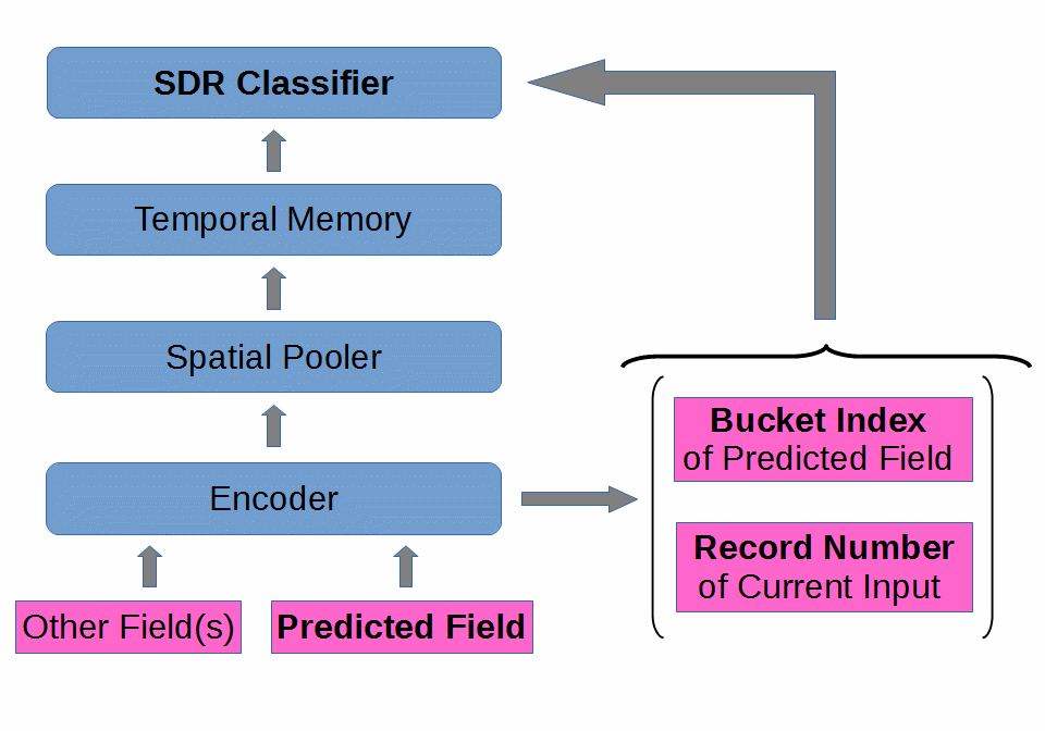
Each time step, the SDR Classifier receives as input a vector of active cells from the Temporal Memory, as well as information about the record number and bucket index used to encode the input from the Encoder.
It may be helpful to see the SDR Classifier in relation to the other modules of an HTM Network:

Suppose we have 3 output units and 5 inputs units (in practice, both of these values would be much larger, especially the number of input units). A schematic of the SDR Classifier would look like this:

(Each input unit is a bit of the activation pattern - the Temporal Memory active cell vector.)
Each Output Unit (OU) receives a weighted sum of the Input Units (IUs) every iteration. There are two stages in this process: 1) weighting 2) summing. I’ll explain weighting first.
Weighting
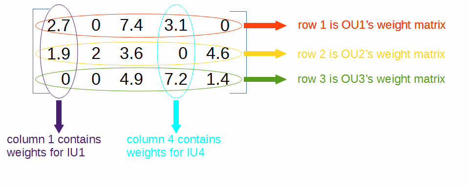
Weighting refers to the process of scaling (multiplying) the value of each IU by some scalar value. The value of an IU will only ever be 1 or 0 (because the Temporal Memory output vector is composed of \(1\)s and \(0\)s, and each IU is a bit of that vector), so we only need to weight the active IUs - those with a value of \(1\). The scalar value we multiply an IU by is called its weight. Each OU maintains its own set of weights - with a particular value stored for each IU. We organize the sets of weights in a matrix.
Using our previous example with 3 OUs and 5 IUs, the weight matrix might look something like:

These weight values change over time, as the SDR Classifier learns. The weights are organized by row (the OU they belong to) and column (the IU they apply to). So, for example, the weight that OU2’s row of the matrix has for IU3 at this point in time is \(3.6\).
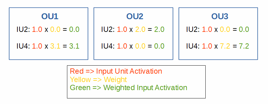
Suppose only IU2 and IU4 are active. This is what the IUs would be weighted as:

Summing
After weighting each of the active IUs, we need to add together all of the weighted inputs for each OU to determine that activation level of each OU:
| IU2 (Weighted) | IU4 (Weighted) | Activation Level | |
| OU1 | 0 | 3.1 | 3.1 |
| OU2 | 2 | 0 | 2 |
| OU3 | 0 | 7.2 | 7.2 |
(In this case the sum is pretty easy, since only two IUs were active, and each OU had a weight of \(0\), but this is rarely the case in practice.)
Weighted Sum Equation
This whole process of computing the weighted sum of the input for each OU to determine their activation levels can be represented/modeled quite handily with the following equation:
\[a_j = \sum_{i=1}^{N}W_{ij}x_i\]Where,
- \(a_j\) is the activation level of the \(j^{th}\) OU.
- \(N\) is the number of IUs (5 in our example).
- \(W_{ij}\) is the weight that the \(j^{th}\) OU is using for the \(i^{th}\) IU (\(i\) is the column in the weight matrix, \(j\) is the row. Some weights in our example include \(0.0, 2.0, 3.1,\) and \(7.2\)).
- \(x_i\) is the state of the \(i^{th}\) IU (either \(1\) or \(0\)).
Written in English, this whole mess just means “We compute the activation level of each OU by weighting each of the IUs (multiplying the state of the IU, either 1 or 0, by its weight, stored in the OU’s row of the weight matrix), and then adding them all together.”
Lets apply the equation to OU2:
\[a_2 = (1.9)(0) + (2)(1) + (3.6)(0) + (4.6)(0) = 2\]Softmaxing the Activation Levels
After computing the activation level of each OU (by doing a weighted sum of the IUs, using that OU’s row of the weight matrix), we need to calculate the probability distribution (likelihood of seeing each class/bucket index from the encoder, a particular number of steps into the future) by exponentiating and normalizing the OUs’ activation levels (doing some math that alters the ratios between the OUs activation levels, and causing them to sum to \(1.0\)). We’ll use the “Softmax” function to do this dirty work for us:
\[y_k = {e^{a_k} \over \sum_{i=1}^{k}e^{a_i}}\]Where,
- \(y_k\) is the probability (\(0 <\leq y_k \leq 1\)) of seeing the \(k^{th}\) class a particular number of steps into the future.
- \(e^{a_k}\) is simply base \(e\approx2.718...\) raised to the activation level of the \(k^{th}\) output unit.
- \(k\) is the number of possible classes (classifications of the input, same thing as the number of buckets used by the encoder, same thing as the number of OUs - so \(k = 3\) in the case of our example).
- \(\sum_{i=1}^{k}e^{a_i}\) is simply the sum of base \(e\) raised to the activation level of each OU.
In plain English, the Softmax function just says “The likelihood of the encoder using the \(k^{th}\) bucket to encode the input a particular number of steps into the future is computed by raising base \(e\) to the activation level of the OU that represents that bucket, and then dividing that value by the sum of base \(e\) raised to the activation level of all the output units.”
A couple of important things to note about the Softmax function:
- Softmax is a non-linear function. This means that the ratios between the activation levels are not preserved. They are intentionally skewed. We could have simply normalized the activation levels, and not exponentiated them. Such a function would look like this: \(y_k = {a_k \over \sum_{i=1}^{k}a_i}\). The exponentiation provided by Softmax is useful, however, because it causes slight differences in activation levels to have large effects on the computed probability distribution, \(y\).
- As a result of using Softmax, our activation levels are normalized such that they sum to \(1.0\). This means that each element of the resulting probability distribution, \(y\) can easily be interpreted as a percentage by multiplying by 100.
See this Tensorflow page for more good information on Softmax.
Let’s use Softmax to compute the probability distribution for seeing each of the possible encoder buckets a particular number of steps in the future. First, lets figure out what the divisor term of Softmax is, \(\sum_{i=1}^{k}e^{a_i}\), since it is going to be the same for each class likelihood we compute:
\[\sum_{i=1}^{k}e^{a_i} = e^{3.1} + e^2 + e^{7.2} = 1369.02\]Now, we’ll evaluate the Softmax function for each class/OU:
\[y_1 = {e^{a_1} \over \sum_{i=1}^{k}e^{a_i}} = {22.2 \over 1369.02} = 0.02\] \[y_2 = {e^{a_2} \over \sum_{i=1}^{k}e^{a_i}} = {7.4 \over 1369.02} = 0.005\] \[y_3 = {e^{a_3} \over \sum_{i=1}^{k}e^{a_i}} = {1339.4 \over 1369.02} = 0.98\]| Class/Bucket Index | Probability |
| \(y_1\) | 0.02 |
| \(y_2\) | 0.005 |
| \(y_3\) | 0.98 |
(I know it doesn’t quite sum to \(1.0\)… I rounded)
Notice the effect of Softmax’s nonlinearity. Recall the activation level (weighted sum of inputs) of OU1 was \(3.1\). The activation level of OU3 was \(7.2\). Thus the ratio of their activation levels is \(0.43\). However, the ratio of their probabilities (after softmaxing their activation levels) is \(0.02\)! That’s a big difference.
These probabilities mean that the SDR Classifier thinks that when the Temporal Memory state (vector of active cells) is 0, 1, 0, 1, 0, that there is a \(2\%\) chance of seeing bucket 1 used to encode the input a particular number of steps in the future, a \({1 \over 5} \%\) chance for bucket 2, and a \(98\%\) chance for bucket 3.
Learning
The SDR Classifier must update its weight matrix in order to learn and make more accurate predictions/inferences. When the SDR Classifier is first initialized, all weights are 0. I’ll now explain how the SDR Classifier proceeds from this starting point.
The SDR Classifier uses a simple learning algorithm to slowly correct its predictions and get close to \(100\%\) accuracy. Each iteration, the SDR Classifier makes a prediction about the input \(n\) steps in the future. This prediction is in the form of a probability distribution. We can represent it like so:
\[y = (y_1, y_2, ... , y_k)\]Where,
- \(y\) is our computed probability distribution.
Each index/element of \(y\) is the likelihood computed by the SDR Classifier of seeing that bucket index used by the encoder. The probability distribution we just computed for our example looks like this:
\[y = (0.02, 0.005, 0.98)\]Each time step we also get a target distribution. This is simply the probability distribution that we want our predicted distribution, \(y\), to match. We can model it like so:
\[z = (z_1, z_2, ... , z_k)\]Where,
- \(z\) is the target distribution.
All of \(z\)’s indexes/elements will be 0, except for one. The “on” element is the one that matches the bucket used by the encoder to encode the input at that time step.
Suppose, using our example, that the encoder used bucket 3. The target distribution for that time step would look like this:
\[z = (0, 0, 1)\]This makes sense. If we tried to predict the input for that time step, this is what we would want our \(y\) to look like. Of course, it probably won’t ever be \(100\%\) accurate, but it can get close, and we did a pretty good job. Our \(y\) was 98% sure we’d see bucket 3 used!
Now then, how does learning work? At time \(t\) we obtain an input to the encoder, and thus a target distribution, \(z\). If we are doing \(5\) step prediction, then we will have received and stored the activation pattern from the Temporal Memory at time \(t-5\). So, we use the stored activation pattern from time \(t-5\) to make a prediction, \(y\). Fortunately for us, we also have the actual input for time \(t\). So we can compare our prediction, \(y\), to the actual target distribution, \(z\), and see how close we were. Then we can adjust out weight matrix, \(W\), to try and make better predictions.
We need to calculate error scores for each index of \(y\). For that, we use the following formula:
\[error_j = z_j - y_j\]This lets us see how good each OU’s prediction is (remember \(j\) indicates the row of the matrix, and each row belongs to one of the OUs). The closer the error is to \(0\) for each OU, the better. An \(error > 0\) means we shot too low, an \(error < 0\) means we were too high.
We multiply the \(error\) by an alpha, \(\alpha\), which lets us speed up or slow down the rate at which the SDR Classifier learns/adapts. The product of this operation is the value we will use to update our matrix:
\[update_j = \alpha(error_j)\](Note that this means each OU gets a single update value, \(update_j\), for all of its columns in the weight matrix, \(W\). Also note that \(\alpha\) must be greater than \(0\), or learning cannot occur.)
Once we have the update value for each \(j\)/matrix-row/OU, we simply go into the weight matrix, \(W\), grab each row, go to each of the columns whose IUs were active at time \(t-5\), and add our update value to whatever weight value exists there already. We can model the whole update process like so:
\[W'_{ij} = W_{ij} + \alpha(z_j - y_j)\]And again, we only do this for the weights that apply to IUs that were active at \(t-5\).
If, for some reason, we wanted to ignore this rule, and update all the IUs’ weights every time step (even ones that were inactive, those whose value was \(0\)), then we could just scale \(update_j\) by \(x_j\). The product will always be \(0\) for nonactive IUs, and remain unchanged for active IUs:
\[W'_{ij} = W_{ij} + x_j(\alpha(z_j - y_j))\]Example Learning Case
Lets use an example case to go through the learning process for a single iteration. We’ll use the following data:
- Predicted Distribution, \(y = (0.1, 0.6, 0.2, 0.1)\)
- Target Distribution, \(z = (0, 1, 0, 0)\)
- Activation Pattern, \(x = (0, 1, 0, 0, 0, 1)\)
- Weight Matrix,
- Alpha, \(\alpha = 0.75\)
First, we compute the error, using \(error_j = z_j - y_j\) :
\[error = (-0.1, 0.4, -0.2, -0.1)\]Next, we scale \(error\)’s elements by \(\alpha\), using \(update_j = \alpha(error_j)\) :
\[update = (-0.075, 0.3, -0.15, -0.075)\]Finally, we update our weight matrix, \(W\), by adding the error signal for each OU to the existing weights for IUs that were active \(n\) steps ago. Our Updated Weight Matrix,
\[\require{color} W' = \begin{bmatrix} 3.5 & \colorbox{red}{3.125} & 0.3 & 4.7 & 2.0 & \colorbox{red}{3.625} \\ 0.0 & \colorbox{green}{5.0} & 2.1 & 3.7 & 1.0 & \colorbox{green}{0.4} \\ 3.2 & \colorbox{red}{2.1} & 3.3 & 1.9 & 0.4 & \colorbox{red}{0.2} \\ 1.1 & \colorbox{red}{2.725} & 3.4 & 1.4 & 0.0 & \colorbox{red}{2.625} \\ \end{bmatrix}\](Weights highlighted red have been lowered. Weights highlighted green have been increased.)
SDR Classifier as a function
It can be helpful to think of the SDR Classifier as a sort of function that given a particular input vector and weight matrix will produce a particular probability distribution.
We can model this function like so:
\[p(C_k\mid x, w) = y_k = {e^{a_k} \over \sum_{i=1}^{k}e^{a_i}}\]Where,
- \(C_k\) represents a particular classification of the input. Each possible classification/class equates to a particular encoder bucket. Each OU represents a single class.
- \(x = (x_1, x_2, ... , x_N)\) represents the sparse binary input vector (a large vector of \(1\)s and \(0\)s, where the majority of elements are \(0\)s).
- \(w = W\) represents our weight matrix at this particular point in time.
- \(p(C_k\mid x, w) = y_k\) represents the Softmaxed probability of seeing the input \(n\) steps in the future encoded as the \(k^{th}\) class. Running this for all possible classifications (all values of \(k\)) produces a complete probability distribution, \(y\).
Notice that this function model does not incorporate the learning process of the SDR Classifier.
Outline of Operations
Just to reiterate and outline the series of operations the SDR Classifier goes through every time step:
- Compute the activation levels for each OU, by performing a weighted sum of the inputs.
- Compute a probability distribution, by applying Softmax to the activation levels.
- Adjust the weight matrix by computing error scores for each of the OUs, and adding them to the appropriate weight matrix elements.
Then we rinse and repeat!
Credits and Thanks
Yuwei Cui and Numenta are responsible for the development of the SDR Classifier.
David Ray, HTM.Java’s lead, was vital to the porting of the SDR Classifier into the HTM.Java codebase.
Mr. Cui from Numenta was kind enough to provide me with these resources:
- Mr. Cui’s personal notes on the SDR Classifier. They were immensely useful in building up my understanding of it.
- A slideshow from California State University, Northridge. Very helpful to understand weight matrices and basics of neural networks.
- A great article written for Google’s Tensorflow project on Softmax Regressions.